
一、机器学习的一些概念
基本概念
- 特征:一组数据的多个属性
- 标签:人为指定特征
- 监督学习:就像分类(离散化的标签),回归(连续性的标签)、【“有标准答案”】
- 无监督学习:就像聚类【“无标准答案”】
- 数据:是机器学习的命脉
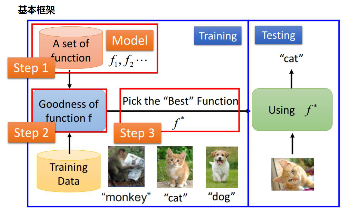
基本框架图
二、机器学习的一些阶段/步骤
sklearn相关提及
- 包含聚类、分类、回归等算法
eg:随机森林、k-means、SVM等 - 包含模型筛选、降维、预处理等算法
- 要特别注意安装该包使用要注意的细节,具体参考上一篇博客
sklearn处理机器学习的一般化sop
- 准备数据集
- 数据分析:(利用np.reshape()成二维(n_samples,n_features))
- 划分数据集:train_test_split()
- 特征工程:特征的提取、特征的归一化nomalization
- 选择模型
- 根据不同场景选择合适的模型:scikit-learn的模型选择路线图
- 分类、聚类、回归……
- 在训练集上训练模型,并调整参数
- 经验选定参数
- 交叉验证确定最优的参数cross validation
- 在测试集上测试模型
- predict预测、score真实值预测值评分、etc
- 保存模型
import pickle
主成分分析:将特征降维
- 统计学相关知识:方差(衡量在一个维度的偏差)、协方差(衡量一个维度是否对另一个维度有影响cov(x,y))
- 线代相关知识:特征值、特征向量、协方差向量
- PCA
三、通过scikit-learn认识机器学习
加载示例数据集
from sklearn import datasets
iris = datasets.load_iris()#用sklearn自身配带的数据
digits = datasets.load_digits()
# C:\Users\wztli\Anaconda3\pkgs\scikit-learn-0.21.3-py37h6288b17_0\Lib\site-packages\sklearn\datasets\data
# 数据集在电脑中的位置
# 查看数据集
# iris
print(iris.data[:5])
print(iris.data.shape)
print(iris.target_names)
print(iris.target)
[[5.1 3.5 1.4 0.2]
 [4.9 3.  1.4 0.2]
 [4.7 3.2 1.3 0.2]
 [4.6 3.1 1.5 0.2]
 [5.  3.6 1.4 0.2]]
(150, 4)
['setosa' 'versicolor' 'virginica']
[0 0 0 0 0 0 0 0 0 0 0 0 0 0 0 0 0 0 0 0 0 0 0 0 0 0 0 0 0 0 0 0 0 0 0 0 0
 0 0 0 0 0 0 0 0 0 0 0 0 0 1 1 1 1 1 1 1 1 1 1 1 1 1 1 1 1 1 1 1 1 1 1 1 1
 1 1 1 1 1 1 1 1 1 1 1 1 1 1 1 1 1 1 1 1 1 1 1 1 1 1 2 2 2 2 2 2 2 2 2 2 2
 2 2 2 2 2 2 2 2 2 2 2 2 2 2 2 2 2 2 2 2 2 2 2 2 2 2 2 2 2 2 2 2 2 2 2 2 2
 2 2]
# digits
print(digits.data)
print(digits.data.shape)
print(digits.target_names)
print(digits.target)
[[ 0.  0.  5. ...  0.  0.  0.]
 [ 0.  0.  0. ... 10.  0.  0.]
 [ 0.  0.  0. ... 16.  9.  0.]
 ...
 [ 0.  0.  1. ...  6.  0.  0.]
 [ 0.  0.  2. ... 12.  0.  0.]
 [ 0.  0. 10. ... 12.  1.  0.]]
(1797, 64)
[0 1 2 3 4 5 6 7 8 9]
[0 1 2 ... 8 9 8]
在训练集上训练模型
# 手动划分训练集、测试集
n_test = 100 # 测试样本个数
train_X = digits.data[:-n_test, :]
train_y = digits.target[:-n_test]

test_X = digits.data[-n_test:, :]
y_true = digits.target[-n_test:]
# 选择SVM模型
from sklearn import svm
svm_model = svm.SVC(gamma=0.001, C=100.)
svm_model = svm.SVC(gamma=100., C=1.)
训练模型
svm_model.fit(train_X, train_y)
#训练要放入两个参数:样本的特征数据,样本的标签
SVC(C=100.0, cache_size=200, class_weight=None, coef0=0.0,
    decision_function_shape='ovr', degree=3, gamma=0.001, kernel='rbf',
    max_iter=-1, probability=False, random_state=None, shrinking=True,
    tol=0.001, verbose=False)
# 选择LR(逻辑回归)模型
from sklearn.linear_model import LogisticRegression
lr_model = LogisticRegression()
训练模型
lr_model.fit(train_X, train_y)
C:\Users\wztli\Anaconda3\lib\site-packages\sklearn\linear_model\logistic.py:432: FutureWarning: Default solver will be changed to 'lbfgs' in 0.22. Specify a solver to silence this warning.
  FutureWarning)
C:\Users\wztli\Anaconda3\lib\site-packages\sklearn\linear_model\logistic.py:469: FutureWarning: Default multi_class will be changed to 'auto' in 0.22. Specify the multi_class option to silence this warning.
  "this warning.", FutureWarning)


LogisticRegression(C=1.0, class_weight=None, dual=False, fit_intercept=True,
                   intercept_scaling=1, l1_ratio=None, max_iter=100,
                   multi_class=’warn’, n_jobs=None, penalty=’l2’,
                   random_state=None, solver=’warn’, tol=0.0001, verbose=0,
                   warm_start=False)
在测试集上测试模型
y_pred_svm = svm_model.predict(test_X)
y_pred_lr = lr_model.predict(test_X)
# 查看结果
# 评价指标
from sklearn.metrics import accuracy_score

#print ‘预测标签:’, y_pred
#print ‘真实标签:’, y_true
print(‘SVM结果:’, accuracy_score(y_true, y_pred_svm))
print(‘LR结果:’, accuracy_score(y_true, y_pred_lr))
SVM结果: 0.98
LR结果: 0.94
保存模型
import pickle

with open(‘svm_model.pkl’, ‘wb’) as f:
    pickle.dump(svm_model, f)
import numpy as np
重新加载模型进行预测
with open(‘svm_model.pkl’, ‘rb’) as f:
model = pickle.load(f)
random_samples_index = np.random.randint(0, 1796, 5)
random_samples = digits.data[random_samples_index, :]
random_targets = digits.target[random_samples_index]
random_predict = model.predict(random_samples)
print(random_predict)
print(random_targets)
[2 2 1 3 8]
[2 2 1 3 8]
四、scikit-learn入门
准备数据集
import numpy as np
from sklearn.model_selection import train_test_split
X = np.random.randint(0, 100, (10, 4))
y = np.random.randint(0, 4, 10)
y.sort()

print(‘样本:’)
print(X)
print(‘标签:’, y)
样本:
[[43 43 18 78]
 [74 24 42 37]
 [36 69 84 47]
 [70 62 77 30]
 [87 38  3 96]
 [68 67 24  7]
 [66 36 72 72]
 [12 94 87 72]
 [66  5 92  6]
 [41 59 60 91]]
标签: [0 0 0 2 2 2 2 3 3 3]
# 分割训练集、测试集
# random_state确保每次随机分割得到相同的结果
X_train, X_test, y_train, y_test = train_test_split(X, y, test_size=1/3., random_state=7)

print(‘训练集:’)
print(X_train)
print(y_train)
print(‘测试集:’)
print(X_test)
print(y_test)
训练集:
[[63 56  7 42]
 [40 47 17 23]
 [41 31 26  8]
 [79 30 22 88]
 [54 85 48 54]
 [89 73 77 41]]
[0 1 1 0 1 1]
测试集:
[[ 3  0 42 86]
 [42 96 83 38]
 [33 45  8 37]
 [ 1 44 75  7]]
[1 1 0 0]
# 特征归一化
from sklearn import preprocessing

x1 = np.random.randint(0, 1000, 5).reshape(5,1)
x2 = np.random.randint(0, 10, 5).reshape(5, 1)
x3 = np.random.randint(0, 100000, 5).reshape(5, 1)
X = np.concatenate([x1, x2, x3], axis=1)
print(X)
[[  353     4 27241]
 [  999     4 34684]
 [  911     4 78606]
 [  310     6 44593]
 [  817     9  6356]]
print(preprocessing.scale(X))
[[-1.12443958 -0.71443451 -0.46550183]
 [ 1.11060033 -0.71443451 -0.15209341]
 [ 0.80613669 -0.71443451  1.69736578]
 [-1.27321159  0.30618622  0.26515287]
 [ 0.48091416  1.83711731 -1.34492342]]
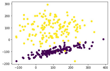
# 生成分类数据进行验证scale的必要性
from sklearn.datasets import make_classification
import matplotlib.pyplot as plt
%matplotlib inline

X, y = make_classification(n_samples=300, n_features=2, n_redundant=0, n_informative=2,
                           random_state=25, n_clusters_per_class=1, scale=100)
plt.scatter(X[:,0], X[:,1], c=y)
plt.show()
from sklearn import svm
注释掉以下这句表示不进行特征归一化
X = preprocessing.scale(X)
X_train, X_test, y_train, y_test = train_test_split(X, y, test_size=1/3., random_state=7)
svm_classifier = svm.SVC()
svm_classifier.fit(X_train, y_train)
svm_classifier.score(X_test, y_test)
C:\Users\wztli\Anaconda3\lib\site-packages\sklearn\svm\base.py:193: FutureWarning: The default value of gamma will change from 'auto' to 'scale' in version 0.22 to account better for unscaled features. Set gamma explicitly to 'auto' or 'scale' to avoid this warning.
  "avoid this warning.", FutureWarning)


0.25
训练模型
# 回归模型
from sklearn import datasets

boston_data = datasets.load_boston()
X = boston_data.data
y = boston_data.target
print(‘样本:’)
print(X[:5, :])
print(‘标签:’)
print(y[:5])
样本:
[[6.3200e-03 1.8000e+01 2.3100e+00 0.0000e+00 5.3800e-01 6.5750e+00
  6.5200e+01 4.0900e+00 1.0000e+00 2.9600e+02 1.5300e+01 3.9690e+02
  4.9800e+00]
 [2.7310e-02 0.0000e+00 7.0700e+00 0.0000e+00 4.6900e-01 6.4210e+00
  7.8900e+01 4.9671e+00 2.0000e+00 2.4200e+02 1.7800e+01 3.9690e+02
  9.1400e+00]
 [2.7290e-02 0.0000e+00 7.0700e+00 0.0000e+00 4.6900e-01 7.1850e+00
  6.1100e+01 4.9671e+00 2.0000e+00 2.4200e+02 1.7800e+01 3.9283e+02
  4.0300e+00]
 [3.2370e-02 0.0000e+00 2.1800e+00 0.0000e+00 4.5800e-01 6.9980e+00
  4.5800e+01 6.0622e+00 3.0000e+00 2.2200e+02 1.8700e+01 3.9463e+02
  2.9400e+00]
 [6.9050e-02 0.0000e+00 2.1800e+00 0.0000e+00 4.5800e-01 7.1470e+00
  5.4200e+01 6.0622e+00 3.0000e+00 2.2200e+02 1.8700e+01 3.9690e+02
  5.3300e+00]]
标签:
[24.  21.6 34.7 33.4 36.2]
# 选择线性回顾模型
from sklearn.linear_model import LinearRegression

lr_model = LinearRegression()
from sklearn.model_selection import train_test_split
分割训练集、测试集
X_train, X_test, y_train, y_test = train_test_split(X, y, test_size=1/3., random_state=7)
# 训练模型
lr_model.fit(X_train, y_train)
LinearRegression(copy_X=True, fit_intercept=True, n_jobs=None, normalize=False)
# 返回参数
lr_model.get_params()
{'copy_X': True, 'fit_intercept': True, 'n_jobs': None, 'normalize': False}
lr_model.score(X_train, y_train)
0.7598132492351114
lr_model.score(X_test, y_test)
0.6693852753319398
交叉验证
from sklearn import datasets
from sklearn.model_selection import train_test_split, cross_val_score
from sklearn.neighbors import KNeighborsClassifier
import matplotlib.pyplot as plt
%matplotlib inline

iris = datasets.load_iris()
X = iris.data
y = iris.target
X_train, X_test, y_train, y_test = train_test_split(X, y, test_size=1/3., random_state=10)
k_range = range(1, 31)
cv_scores = []
for n in k_range:
    knn = KNeighborsClassifier(n)
    scores = cross_val_score(knn, X_train, y_train, cv=10, scoring=’accuracy’) # 分类问题使用
    #scores = cross_val_score(knn, X_train, y_train, cv=10, scoring=’neg_mean_squared_error’) # 回归问题使用
    cv_scores.append(scores.mean())
plt.plot(k_range, cv_scores)
plt.xlabel(‘K’)
plt.ylabel(‘Accuracy’)
plt.show()
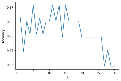
# 选择最优的K
best_knn = KNeighborsClassifier(n_neighbors=5)
best_knn.fit(X_train, y_train)
print(best_knn.score(X_test, y_test))
print(best_knn.predict(X_test))
0.96
[1 2 0 1 0 1 2 1 0 1 1 2 1 0 0 2 1 0 0 0 2 2 2 0 1 0 1 1 1 2 1 1 2 2 2 0 2
 2 2 2 0 0 1 0 1 0 1 2 2 2]
参考
- scikit-learn中文文档github文中链接为英文文档
- 解释iris数据集
评论区